Tag Archives: Cartography

Mapping Mule’s Ears

One common factor contributing to mistakes when people are identifying plants is the scarcity of user-friendly visual documentation (i.e., maps) showing where different species occur in the world. Sure, more than one species of a genus will often co-occur in the same general area, but maps can help you quickly narrow down the number of possibilities in a given area.

Another aid that’s commonly missing is an explanation of how one species differs from a small set of related or similar species, where they may occur near each other. Keys can provide the technical details for distinguishing one plant from all others in a genus-wide or family-wide context, often over a wide area, but may obscure the simple details that can distinguish “Species A” from “Species D” where just those two happen to occur together.

How nice it would be to have more maps of species distributions based on current data for collections and observations. Such maps, together with keys and notes on how to distinguish one species from others in the same area, could facilitate more accurate identifications—especially in genera with little to moderate overlap of species ranges.

Wyethia mollis

This could be a fun project to help pass a pandemic winter, yes?

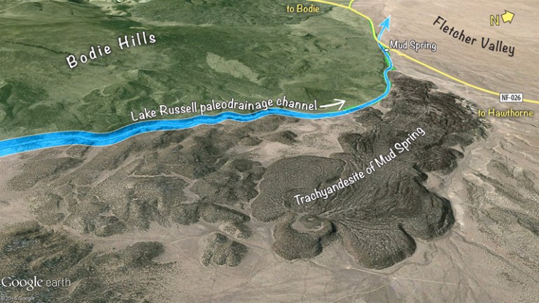
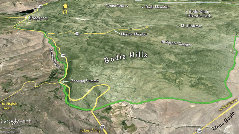
To explore the idea a bit further, I looked for a genus of modest size in western North America, with at least one species in Mono County. There are many genera to choose from. I selected Wyethia, commonly known as Mule’s Ears (or Mule Ears or Mules Ears), a genus with 14 distinct and well-documented species scattered across the mountains, hills, and deserts of western North America. Hikers in the upper elevations and east side of the Sierra Nevada will know Woolly Mule’s Ears (Wyethia mollis) as one of the brightest and showiest sunflowers of the region.

Here, then, is Mule’s Ears: an Atlas and Guide, a free PDF on my Downloads page. Look it over and let me know if you find this approach and format useful (corrections and suggestions are always welcome).

A Note on Taxonomy
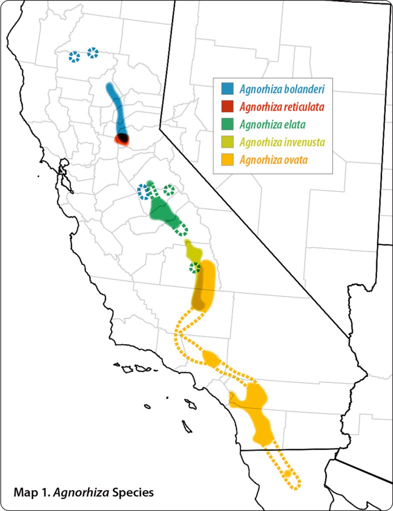
Traditionally, the 14 species of Mule’s Ears have been grouped all together in the genus Wyethia. (As of this date, the Jepson eFlora still treats all California species under Wyethia.) Currently, however, most sources recognize 3 separate genera in this group: Wyethia in a stricter sense (with 8 species), Agnorhiza (with 5 species), and Scabrethia (with 1 species). These are differentiated mostly by the shape, relative sizes, and distribution of leaves. Personally, I’m not always a fan of splitting genera by their sections, but in this case, I think it helps us recognize very visible differences within the group and makes the keys more manageable.

Methods
I downloaded location data (in CSV format) for herbarium collections of each species from the California Consortium of Herbaria (CCH), the Southwest Environmental Information Network (SEINet), the Intermountain Regional Herbarium Network, and the Consortium of Pacific Northwest Herbaria, along with crowd-sourced observation data from iNaturalist. These I imported to a base map of US states and counties, Canadian provinces, and Mexican states using QGIS (a free, open source GIS application).

For each species I exported a PDF dot map of collections and observations. These I placed into Adobe Illustrator, aligned with a clean base of only the state and county boundaries. I then traced the approximate boundaries of the occurrence clouds. In doing so, I did quick reality checks on occurrences that appeared inconsistent with overall distribution patterns or distributions reported in the literature. Many of these anomalies turned out to be obvious misidentifications or incorrect mapping of collection coordinates. Colors and patterns were used to differentiate species in the maps.

The final booklet, together with photographs licensed for non-commercial use by iNaturalist contributors (acknowledged in the booklet), was assembled in Adobe InDesign.

How to use this Booklet
1. Download the 16-page PDF from the DOWNLOADS PAGE. I suggest saving this into the library of the books app on your smart phone or tablet (e.g., Books on Apple devices) to keep it handy in the field. The pages are formatted as half-letter size (5.5 X 8.5 inches), so it’s fairly readable on your phone (if you’re near-sighted) or on your tablet.

2. You can also print this as a 16-page booklet from your computer using Adobe Acrobat or Adobe Reader (and probably other PDF apps). Tell the application to print all pages in Booklet format, both sides, left binding, and auto-rotate pages. Use letter-size (8.5 X 11) paper, and select your specific printer (not the generic “Any Printer”) and “US Letter” paper size in the printer dialog. This should result in the pages being filled and with centers properly aligned for folding. After printing, arrange as needed to make sure the page numbers are in proper sequence, fold the stack in the middle, and staple along the fold (a long-reach stapler works best for this).

3. Go forth and Botanize!


Copyright © Tim Messick 2022. All rights reserved.

How Big are the Bodie Hills?

How big are the Bodie Hills? How many square miles? That depends, but first, here are the numbers I’ve come up with:

  • in Mono, CA . . . . . . . . . . . .259 square miles (62%)
  • in Mineral, NV . . . . . . . . . .146 square miles (35%)
  • in Lyon, NV . . . . . . . . . . . . . 12 square miles (3%)
  • Total area . . . . . . . . . . . . . . . . 417 square miles

Overview of the Bodie Hills

Overview of the Bodie Hills from the southeast

It depends, of course, on where you draw the boundaries. There are relatively sharp natural boundaries in some areas — Virginia Creek along the southwest edge, the East Walker River in the canyon that separates the Bodie Hills from the Sweetwater Mountains, and the edge of Big Meadows south of Bridgeport.

In other areas the natural or physical boundary is less obvious. Along the east side of the range, the channels of Rough Creek and Mud Spring Wash are potential boundaries, but that would include a good bit of Fletcher Valley, with lower elevations and different vegetation than in the Bodie Hills proper. Along the south edge of the range, there is a relatively narrow transition in some areas from the rocky and wooded Bodie Hills to the sandy, mostly shrubby Mono Basin. But there’s no single elevation contour that consistently follows this transition, and the boundary becomes more vague east of Trench Canyon.

Should Cedar Hill (about 12 square miles) be included? I’ve left it outside the Bodie Hills, running the boundary instead through Trench Canyon, but that choice is fairly arbitrary.

Should the very young (<100,000 year-old) late Pleistocene trachyandesite of Mud Spring—the lava dome that fills the narrow far-southeast end of Fletcher Valley—be included? I’ve left it out, following instead the approximate route of the paleodrainage channel of Lake Russell (Pleistocene Mono Lake), along the southern edge of that formation.

Bodie Hills from the east

Bodie Hills from the east

Should boundary follow the East Walker River through the irrigated valley bottom just east of the state line? I’ve drawn it closer to the base of the hill slopes to the south, mostly excluding that valley bottom.

Bodie Hills from the north

Bodie Hills from the north

In some areas lacking a hard “edge” to the Bodie Hills, roads provide a convenient, if somewhat arbitrary boundary. My southern boundary follows roads from US 395 to Cottonwood Canyon. My eastern boundary follows roads in the vicinity of Alkali Lake and in Fletcher Valley from about Mud Spring to the Miocene trachyandesites incised by lower Rough Creek. For convenience, my western boundary follows US 395 south of Bridgeport and State Route 182 north of Bridgeport.

Bodie Hills from the southwest

Bodie Hills from the southwest

One could quibble and fuss over the boundary in a number of places, but further refinement would change the total area (and the number of plants included in the checklist) very little.

Methods: I imported 13 US Topo quadrangles (1:24,000 scale) covering the Bodie Hills into Adobe Illustrator, using Avenza’s MAPublisher plug-in to maintain the georeferencing from the GeoPDFs made by USGS. I drew and adjusted the boundaries described above for the entire range on a new georeferenced layer, copying and joining road and river line segments from other layers where available. I then divided that area using the county boundary lines. I exported the three resulting shapes to a KMZ file, opened that in Google Earth Pro, and looked at the their “measurements” info for the square miles in each county.


Copyright © Tim Messick 2016. All rights reserved.
DOWNLOAD THE CHECKLIST

Mapping Monitor Pass

This is one of those posts about a place somewhat “beyond” the Bodie Hills. But there is a connection: when traveling to the Bodie Hills, I often travel across Monitor Pass, on State Route 89 in Alpine County, east of Markleeville. It’s a wonderfully scenic and botanically interesting area — one of my favorite places along the route to Mono County. Earlier this year I started making a map of the Monitor Pass area (during some spare hours at the office) as a way of getting to know the area better.

Monitor Pass and Vicinity, from Markleeville to Topaz (click to enlarge, back to return):

Monitor Pass and Vicinity

But then the Washington Fire happened. According to InciWeb, the fire incident information system, it was ignited by lightning sometime in early June, but remained small and undetected until June 19, 2015. Between then and the first week of July, nearly 17,800 acres of pine forest and sagebrush scrub burned in the East Fork Carson River watershed between Markleeville and Monitor Pass. Nearly 1200 personnel worked hard to bring the fire under control. They prevented damage to the small city of Markleeville and many nearby recreational sites. Remarkably, they got the  Monitor Pass and Ebbetts Pass roads open and safe to use in time for the annual “Death Ride” on July 11 — a grueling, high-profile, high-altitude cycling event with 5 mountain pass ascents over a course of 129 miles.

So my map of a favorite driving route turned into a fire history map of the Monitor Pass area. I downloaded the final perimeter of the Washington Fire (a KML file available from InciWeb). Then I found a statewide fire history geodatabase from the California Fire and Resource Assessment Program (FRAP) that maps incidents as far back as 1878, though the earliest fire mapped in the Monitor Pass area is 1941.

Fire history map of the Monitor Pass area (click to enlarge, back to return):

Monitor Pass Area Fire History

Fires have very long-lasting effects in this region of steep, arid topography. Pines, junipers, sagebrush and other large woody shrubs take many decades to recover even to a fraction of the cover that was present before a large fire. Areas that burned east of Monitor Pass in 2004 still have little woody vegetation. Areas that burned in the ’70s, ’80s, and ’90s are still clearly visible from the air, in Google Earth, or on the ground. Vegetative biomass and the wildlife habitat it provides takes a very long time to recover.

Washington Fire

Washington Fire burn area, near Heenan Lake, 7/12/2015

Washington Fire

Washington Fire perimeter, near Heenan Lake, 7/12/2015

The maps were compiled in Adobe Illustrator with the Avenza MAPublisher plug-in from GIS data available on the internet. The shaded relief background was created in Adobe Photoshop with the Avenza Geographic Imager plug-in and digital elevation data available from USGS.

MarkleevilleAfter the fire, in Markleeville


Copyright © Tim Messick 2015. All rights reserved.